Polynomial Regression Using TensorFlow

In this tutorial you will learn about polynomial regression and how you can implement it in Tensorflow.

In this, we will be performing polynomial regression using 5 types of equations -

Linear
Quadratic
Cubic
Quartic
Quintic

Regression

What is Regression?

Regression is a statistical measurement that is used to try to determine the relationship between a dependent variable (often denoted by Y), and series of varying variables (called independent variables, often denoted by X ).

What is Polynomial Regression

This is a form of Regression Analysis where the relationship between Y and X is denoted as the nth degree/power of X. Polynomial regression even fits a non-linear relationship (e.g when the points don't form a straight line).

Imports

import tensorflow.compat.v1 as tf
tf.disable_v2_behavior()
import matplotlib.pyplot as plt
import numpy as np
import pandas as pd

Dataset

Creating Random Data

Even though in this tutorial we will use a Position Vs Salary dataset, it is important to know how to create synthetic data

To create 50 values spaced evenly between 0 and 50, we use NumPy's linspace function

linspace(lower_limit, upper_limit, no_of_observations)

x = np.linspace(0, 50, 50)
y = np.linspace(0, 50, 50)

We use the following function to add noise to the data, so that our values

x += np.random.uniform(-4, 4, 50)
y += np.random.uniform(-4, 4, 50)

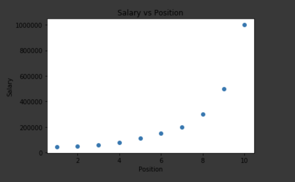
Position vs Salary Dataset

We will be using https://drive.google.com/file/d/1tNL4jxZEfpaP4oflfSn6pIHJX7Pachm9/view (Salary vs Position Dataset)

!wget --no-check-certificate 'https://docs.google.com/uc?export=download&id=1tNL4jxZEfpaP4oflfSn6pIHJX7Pachm9' -O data.csv

df = pd.read_csv("data.csv")

df # this gives us a preview of the dataset we are working with

| Position          | Level | Salary  |
|-------------------|-------|---------|
| Business Analyst  | 1     | 45000   |
| Junior Consultant | 2     | 50000   |
| Senior Consultant | 3     | 60000   |
| Manager           | 4     | 80000   |
| Country Manager   | 5     | 110000  |
| Region Manager    | 6     | 150000  |
| Partner           | 7     | 200000  |
| Senior Partner    | 8     | 300000  |
| C-level           | 9     | 500000  |
| CEO               | 10    | 1000000 |

We convert the salary column as the ordinate (y-coordinate) and level column as the abscissa

abscissa = df["Level"].to_list() # abscissa = [1,2,3,4,5,6,7,8,9,10]
ordinate = df["Salary"].to_list() # ordinate = [45000,50000,60000,80000,110000,150000,200000,300000,500000,1000000]

n = len(abscissa) # no of observations
plt.scatter(abscissa, ordinate)
plt.ylabel('Salary')
plt.xlabel('Position')
plt.title("Salary vs Position")
plt.show()

Defining Stuff

X = tf.placeholder("float")
Y = tf.placeholder("float")

Defining Variables

We first define all the coefficients and constant as tensorflow variables having a random initial value

a = tf.Variable(np.random.randn(), name = "a")
b = tf.Variable(np.random.randn(), name = "b")
c = tf.Variable(np.random.randn(), name = "c")
d = tf.Variable(np.random.randn(), name = "d")
e = tf.Variable(np.random.randn(), name = "e")
f = tf.Variable(np.random.randn(), name = "f")

Model Configuration

learning_rate = 0.2
no_of_epochs = 25000

Equations

deg1 = a*X + b
deg2 = a*tf.pow(X,2) + b*X + c
deg3 = a*tf.pow(X,3) + b*tf.pow(X,2) + c*X + d
deg4 = a*tf.pow(X,4) + b*tf.pow(X,3) + c*tf.pow(X,2) + d*X + e
deg5 = a*tf.pow(X,5) + b*tf.pow(X,4) + c*tf.pow(X,3) + d*tf.pow(X,2) + e*X + f

Cost Function

We use the Mean Squared Error Function

mse1 = tf.reduce_sum(tf.pow(deg1-Y,2))/(2*n)
mse2 = tf.reduce_sum(tf.pow(deg2-Y,2))/(2*n)
mse3 = tf.reduce_sum(tf.pow(deg3-Y,2))/(2*n)
mse4 = tf.reduce_sum(tf.pow(deg4-Y,2))/(2*n)
mse5 = tf.reduce_sum(tf.pow(deg5-Y,2))/(2*n)

Optimizer

We use the AdamOptimizer for the polynomial functions and GradientDescentOptimizer for the linear function

optimizer1 = tf.train.GradientDescentOptimizer(learning_rate).minimize(mse1)
optimizer2 = tf.train.AdamOptimizer(learning_rate).minimize(mse2)
optimizer3 = tf.train.AdamOptimizer(learning_rate).minimize(mse3)
optimizer4 = tf.train.AdamOptimizer(learning_rate).minimize(mse4)
optimizer5 = tf.train.AdamOptimizer(learning_rate).minimize(mse5)

init=tf.global_variables_initializer()

Model Predictions

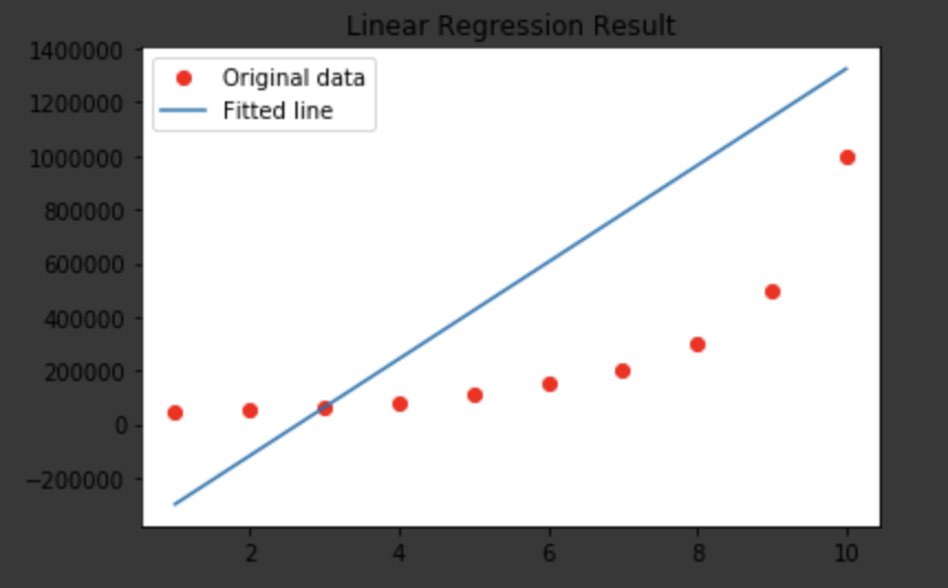
For each type of equation first we make the model predict the values of the coefficient(s) and constant, once we get these values we use it to predict the Y values using the X values. We then plot it to compare the actual data and predicted line.

Linear Equation

with tf.Session() as sess:
    sess.run(init)
    for epoch in range(no_of_epochs):
      for (x,y) in zip(abscissa, ordinate):
        sess.run(optimizer1, feed_dict={X:x, Y:y})
      if (epoch+1)%1000==0:
        cost = sess.run(mse1,feed_dict={X:abscissa,Y:ordinate})
        print("Epoch",(epoch+1), ": Training Cost:", cost," a,b:",sess.run(a),sess.run(b))

        training_cost = sess.run(mse1,feed_dict={X:abscissa,Y:ordinate})
        coefficient1 = sess.run(a)
        constant = sess.run(b)

print(training_cost, coefficient1, constant)

Epoch 1000 : Training Cost: 88999125000.0  a,b: 180396.42 -478869.12
Epoch 2000 : Training Cost: 88999125000.0  a,b: 180396.42 -478869.12
Epoch 3000 : Training Cost: 88999125000.0  a,b: 180396.42 -478869.12
Epoch 4000 : Training Cost: 88999125000.0  a,b: 180396.42 -478869.12
Epoch 5000 : Training Cost: 88999125000.0  a,b: 180396.42 -478869.12
Epoch 6000 : Training Cost: 88999125000.0  a,b: 180396.42 -478869.12
Epoch 7000 : Training Cost: 88999125000.0  a,b: 180396.42 -478869.12
Epoch 8000 : Training Cost: 88999125000.0  a,b: 180396.42 -478869.12
Epoch 9000 : Training Cost: 88999125000.0  a,b: 180396.42 -478869.12
Epoch 10000 : Training Cost: 88999125000.0  a,b: 180396.42 -478869.12
Epoch 11000 : Training Cost: 88999125000.0  a,b: 180396.42 -478869.12
Epoch 12000 : Training Cost: 88999125000.0  a,b: 180396.42 -478869.12
Epoch 13000 : Training Cost: 88999125000.0  a,b: 180396.42 -478869.12
Epoch 14000 : Training Cost: 88999125000.0  a,b: 180396.42 -478869.12
Epoch 15000 : Training Cost: 88999125000.0  a,b: 180396.42 -478869.12
Epoch 16000 : Training Cost: 88999125000.0  a,b: 180396.42 -478869.12
Epoch 17000 : Training Cost: 88999125000.0  a,b: 180396.42 -478869.12
Epoch 18000 : Training Cost: 88999125000.0  a,b: 180396.42 -478869.12
Epoch 19000 : Training Cost: 88999125000.0  a,b: 180396.42 -478869.12
Epoch 20000 : Training Cost: 88999125000.0  a,b: 180396.42 -478869.12
Epoch 21000 : Training Cost: 88999125000.0  a,b: 180396.42 -478869.12
Epoch 22000 : Training Cost: 88999125000.0  a,b: 180396.42 -478869.12
Epoch 23000 : Training Cost: 88999125000.0  a,b: 180396.42 -478869.12
Epoch 24000 : Training Cost: 88999125000.0  a,b: 180396.42 -478869.12
Epoch 25000 : Training Cost: 88999125000.0  a,b: 180396.42 -478869.12
88999125000.0 180396.42 -478869.12

predictions = []
for x in abscissa:
  predictions.append((coefficient1*x + constant))
plt.plot(abscissa , ordinate, 'ro', label ='Original data')
plt.plot(abscissa, predictions, label ='Fitted line')
plt.title('Linear Regression Result')
plt.legend()
plt.show()

Quadratic Equation

with tf.Session() as sess:
    sess.run(init)
    for epoch in range(no_of_epochs):
      for (x,y) in zip(abscissa, ordinate):
        sess.run(optimizer2, feed_dict={X:x, Y:y})
      if (epoch+1)%1000==0:
        cost = sess.run(mse2,feed_dict={X:abscissa,Y:ordinate})
        print("Epoch",(epoch+1), ": Training Cost:", cost," a,b,c:",sess.run(a),sess.run(b),sess.run(c))

        training_cost = sess.run(mse2,feed_dict={X:abscissa,Y:ordinate})
        coefficient1 = sess.run(a)
        coefficient2 = sess.run(b)
        constant = sess.run(c)

print(training_cost, coefficient1, coefficient2, constant)

Epoch 1000 : Training Cost: 52571360000.0  a,b,c: 1002.4456 1097.0197 1276.6921
Epoch 2000 : Training Cost: 37798890000.0  a,b,c: 1952.4263 2130.2825 2469.7756
Epoch 3000 : Training Cost: 26751185000.0  a,b,c: 2839.5825 3081.6118 3554.351
Epoch 4000 : Training Cost: 19020106000.0  a,b,c: 3644.56 3922.9563 4486.3135
Epoch 5000 : Training Cost: 14060446000.0  a,b,c: 4345.042 4621.4233 5212.693
Epoch 6000 : Training Cost: 11201084000.0  a,b,c: 4921.1855 5148.1504 5689.0713
Epoch 7000 : Training Cost: 9732740000.0  a,b,c: 5364.764 5493.0156 5906.754
Epoch 8000 : Training Cost: 9050918000.0  a,b,c: 5685.4067 5673.182 5902.0728
Epoch 9000 : Training Cost: 8750394000.0  a,b,c: 5906.9814 5724.8906 5734.746
Epoch 10000 : Training Cost: 8613128000.0  a,b,c: 6057.3677 5687.3364 5461.167
Epoch 11000 : Training Cost: 8540034600.0  a,b,c: 6160.547 5592.3022 5122.8633
Epoch 12000 : Training Cost: 8490983000.0  a,b,c: 6233.9175 5462.025 4747.111
Epoch 13000 : Training Cost: 8450816500.0  a,b,c: 6289.048 5310.7583 4350.6997
Epoch 14000 : Training Cost: 8414082000.0  a,b,c: 6333.199 5147.394 3943.9294
Epoch 15000 : Training Cost: 8378841600.0  a,b,c: 6370.7944 4977.1704 3532.476
Epoch 16000 : Training Cost: 8344471000.0  a,b,c: 6404.468 4803.542 3120.2087
Epoch 17000 : Training Cost: 8310785500.0  a,b,c: 6435.365 4628.1523 2709.1445
Epoch 18000 : Training Cost: 8277482000.0  a,b,c: 6465.5493 4451.833 2300.2783
Epoch 19000 : Training Cost: 8244650000.0  a,b,c: 6494.609 4274.826 1894.3738
Epoch 20000 : Training Cost: 8212349000.0  a,b,c: 6522.8247 4098.1733 1491.9915
Epoch 21000 : Training Cost: 8180598300.0  a,b,c: 6550.6567 3922.7405 1093.3868
Epoch 22000 : Training Cost: 8149257700.0  a,b,c: 6578.489 3747.8362 698.53357
Epoch 23000 : Training Cost: 8118325000.0  a,b,c: 6606.1973 3573.2742 307.3541
Epoch 24000 : Training Cost: 8088001000.0  a,b,c: 6632.96 3399.878 -79.89219
Epoch 25000 : Training Cost: 8058094600.0  a,b,c: 6659.793 3227.2517 -463.03156
8058094600.0 6659.793 3227.2517 -463.03156

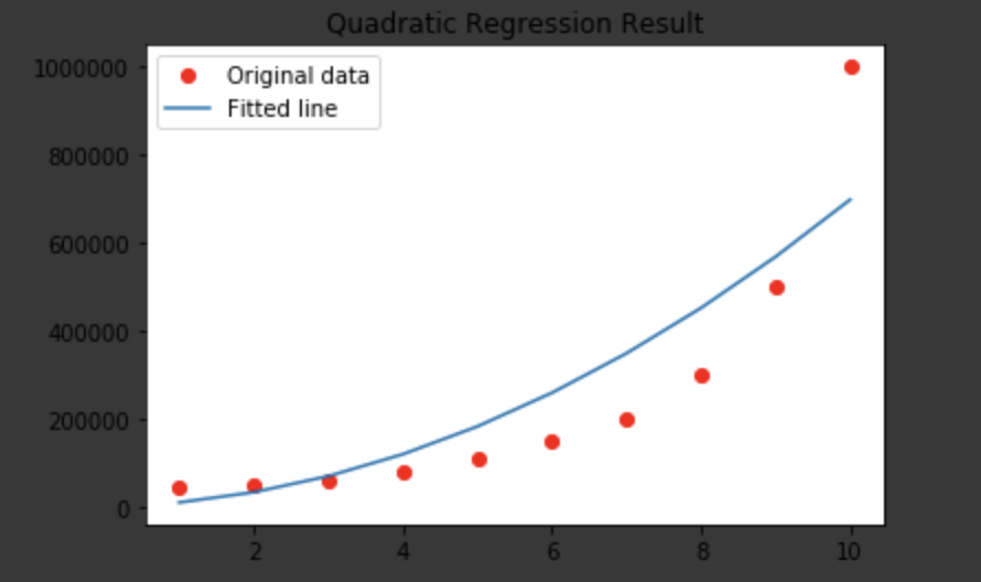
predictions = []
for x in abscissa:
  predictions.append((coefficient1*pow(x,2) + coefficient2*x + constant))
plt.plot(abscissa , ordinate, 'ro', label ='Original data')
plt.plot(abscissa, predictions, label ='Fitted line')
plt.title('Quadratic Regression Result')
plt.legend()
plt.show()

Cubic

with tf.Session() as sess:
    sess.run(init)
    for epoch in range(no_of_epochs):
      for (x,y) in zip(abscissa, ordinate):
        sess.run(optimizer3, feed_dict={X:x, Y:y})
      if (epoch+1)%1000==0:
        cost = sess.run(mse3,feed_dict={X:abscissa,Y:ordinate})
        print("Epoch",(epoch+1), ": Training Cost:", cost," a,b,c,d:",sess.run(a),sess.run(b),sess.run(c),sess.run(d))

        training_cost = sess.run(mse3,feed_dict={X:abscissa,Y:ordinate})
        coefficient1 = sess.run(a)
        coefficient2 = sess.run(b)
        coefficient3 = sess.run(c)
        constant = sess.run(d)

print(training_cost, coefficient1, coefficient2, coefficient3, constant)

Epoch 1000 : Training Cost: 4279814000.0  a,b,c,d: 670.1527 694.4212 751.4653 903.9527
Epoch 2000 : Training Cost: 3770950400.0  a,b,c,d: 742.6414 666.3489 636.94525 859.2088
Epoch 3000 : Training Cost: 3717708300.0  a,b,c,d: 756.2582 569.3339 448.105 748.23956
Epoch 4000 : Training Cost: 3667464000.0  a,b,c,d: 769.4476 474.0318 265.5761 654.75525
Epoch 5000 : Training Cost: 3620040700.0  a,b,c,d: 782.32324 380.54272 89.39888 578.5136
Epoch 6000 : Training Cost: 3575265800.0  a,b,c,d: 794.8898 288.83356 -80.5215 519.13654
Epoch 7000 : Training Cost: 3532972000.0  a,b,c,d: 807.1608 198.87044 -244.31102 476.2061
Epoch 8000 : Training Cost: 3493009200.0  a,b,c,d: 819.13513 110.64169 -402.0677 449.3291
Epoch 9000 : Training Cost: 3455228400.0  a,b,c,d: 830.80255 24.0964 -553.92804 438.0652
Epoch 10000 : Training Cost: 3419475500.0  a,b,c,d: 842.21594 -60.797424 -700.0123 441.983
Epoch 11000 : Training Cost: 3385625300.0  a,b,c,d: 853.3363 -144.08699 -840.467 460.6356
Epoch 12000 : Training Cost: 3353544700.0  a,b,c,d: 864.19135 -225.8125 -975.4196 493.57703
Epoch 13000 : Training Cost: 3323125000.0  a,b,c,d: 874.778 -305.98932 -1104.9867 540.39465
Epoch 14000 : Training Cost: 3294257000.0  a,b,c,d: 885.1007 -384.63474 -1229.277 600.65607
Epoch 15000 : Training Cost: 3266820000.0  a,b,c,d: 895.18823 -461.819 -1348.4417 673.9051
Epoch 16000 : Training Cost: 3240736000.0  a,b,c,d: 905.0128 -537.541 -1462.6171 759.7118
Epoch 17000 : Training Cost: 3215895000.0  a,b,c,d: 914.60065 -611.8676 -1571.9058 857.6638
Epoch 18000 : Training Cost: 3192216800.0  a,b,c,d: 923.9603 -684.8093 -1676.4642 967.30475
Epoch 19000 : Training Cost: 3169632300.0  a,b,c,d: 933.08594 -756.3582 -1776.4275 1088.2198
Epoch 20000 : Training Cost: 3148046300.0  a,b,c,d: 941.9928 -826.6257 -1871.9355 1219.9702
Epoch 21000 : Training Cost: 3127394800.0  a,b,c,d: 950.67896 -895.6205 -1963.0989 1362.1665
Epoch 22000 : Training Cost: 3107608600.0  a,b,c,d: 959.1487 -963.38116 -2050.0586 1514.4026
Epoch 23000 : Training Cost: 3088618200.0  a,b,c,d: 967.4355 -1029.9625 -2132.961 1676.2717
Epoch 24000 : Training Cost: 3070361300.0  a,b,c,d: 975.52875 -1095.4292 -2211.854 1847.4485
Epoch 25000 : Training Cost: 3052791300.0  a,b,c,d: 983.4346 -1159.7922 -2286.9412 2027.4857
3052791300.0 983.4346 -1159.7922 -2286.9412 2027.4857

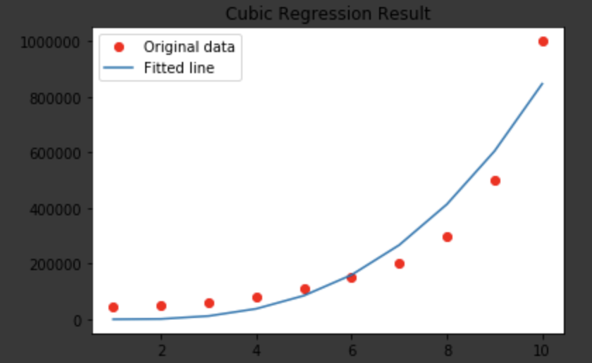
predictions = []
for x in abscissa:
  predictions.append((coefficient1*pow(x,3) + coefficient2*pow(x,2) + coefficient3*x + constant))
plt.plot(abscissa , ordinate, 'ro', label ='Original data')
plt.plot(abscissa, predictions, label ='Fitted line')
plt.title('Cubic Regression Result')
plt.legend()
plt.show()

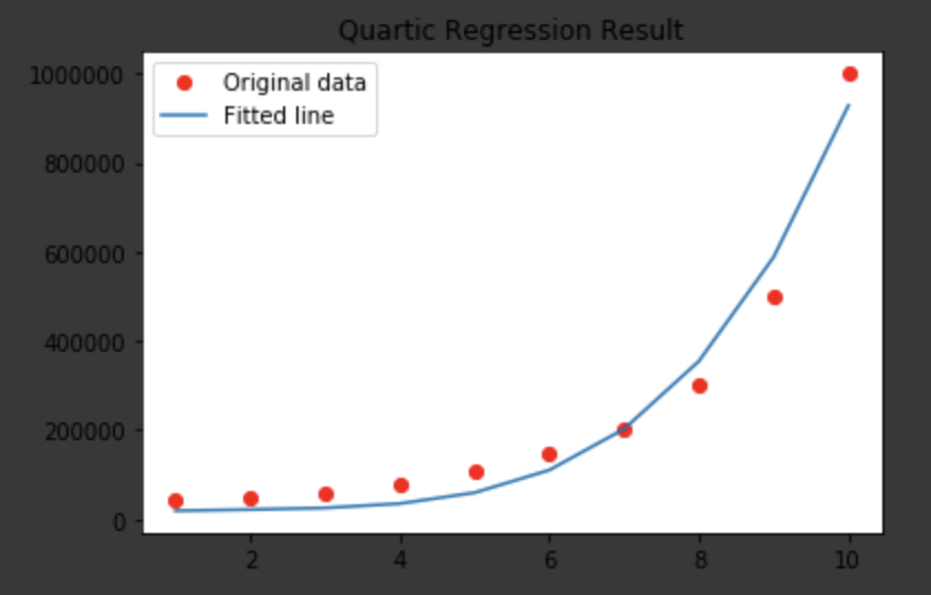
Quartic

with tf.Session() as sess:
    sess.run(init)
    for epoch in range(no_of_epochs):
      for (x,y) in zip(abscissa, ordinate):
        sess.run(optimizer4, feed_dict={X:x, Y:y})
      if (epoch+1)%1000==0:
        cost = sess.run(mse4,feed_dict={X:abscissa,Y:ordinate})
        print("Epoch",(epoch+1), ": Training Cost:", cost," a,b,c,d:",sess.run(a),sess.run(b),sess.run(c),sess.run(d),sess.run(e))

        training_cost = sess.run(mse4,feed_dict={X:abscissa,Y:ordinate})
        coefficient1 = sess.run(a)
        coefficient2 = sess.run(b)
        coefficient3 = sess.run(c)
        coefficient4 = sess.run(d)
        constant = sess.run(e)

print(training_cost, coefficient1, coefficient2, coefficient3, coefficient4, constant)

Epoch 1000 : Training Cost: 1902632600.0  a,b,c,d: 84.48304 52.210594 54.791424 142.51952 512.0343
Epoch 2000 : Training Cost: 1854316200.0  a,b,c,d: 88.998955 13.073557 14.276088 223.55667 1056.4655
Epoch 3000 : Training Cost: 1812812400.0  a,b,c,d: 92.9462 -22.331177 -15.262934 327.41858 1634.9054
Epoch 4000 : Training Cost: 1775716000.0  a,b,c,d: 96.42522 -54.64535 -35.829437 449.5028 2239.1392
Epoch 5000 : Training Cost: 1741494100.0  a,b,c,d: 99.524734 -84.43976 -49.181057 585.85876 2862.4915
Epoch 6000 : Training Cost: 1709199600.0  a,b,c,d: 102.31984 -112.19895 -56.808075 733.1876 3499.6199
Epoch 7000 : Training Cost: 1678261800.0  a,b,c,d: 104.87324 -138.32709 -59.9442 888.79626 4146.2944
Epoch 8000 : Training Cost: 1648340600.0  a,b,c,d: 107.23536 -163.15173 -59.58964 1050.524 4798.979
Epoch 9000 : Training Cost: 1619243400.0  a,b,c,d: 109.44742 -186.9409 -56.53944 1216.6432 5454.9463
Epoch 10000 : Training Cost: 1590821900.0  a,b,c,d: 111.54233 -209.91287 -51.423084 1385.8513 6113.5137
Epoch 11000 : Training Cost: 1563042200.0  a,b,c,d: 113.54405 -232.21953 -44.73371 1557.1084 6771.7046
Epoch 12000 : Training Cost: 1535855600.0  a,b,c,d: 115.471565 -253.9838 -36.851135 1729.535 7429.069
Epoch 13000 : Training Cost: 1509255300.0  a,b,c,d: 117.33939 -275.29697 -28.0714 1902.5308 8083.9634
Epoch 14000 : Training Cost: 1483227000.0  a,b,c,d: 119.1605 -296.2472 -18.618649 2075.6094 8735.381
Epoch 15000 : Training Cost: 1457726700.0  a,b,c,d: 120.94584 -316.915 -8.650095 2248.3247 9384.197
Epoch 16000 : Training Cost: 1432777300.0  a,b,c,d: 122.69806 -337.30704 1.7027153 2420.5771 10028.871
Epoch 17000 : Training Cost: 1408365000.0  a,b,c,d: 124.42179 -357.45245 12.33499 2592.2983 10669.157
Epoch 18000 : Training Cost: 1384480000.0  a,b,c,d: 126.12332 -377.39734 23.168756 2763.0933 11305.027
Epoch 19000 : Training Cost: 1361116800.0  a,b,c,d: 127.80568 -397.16415 34.160156 2933.0452 11935.669
Epoch 20000 : Training Cost: 1338288100.0  a,b,c,d: 129.4674 -416.72803 45.259155 3101.7727 12561.179
Epoch 21000 : Training Cost: 1315959700.0  a,b,c,d: 131.11403 -436.14285 56.4436 3269.3142 13182.058
Epoch 22000 : Training Cost: 1294164700.0  a,b,c,d: 132.74377 -455.3779 67.6757 3435.3833 13796.807
Epoch 23000 : Training Cost: 1272863600.0  a,b,c,d: 134.35779 -474.45316 78.96117 3600.264 14406.58
Epoch 24000 : Training Cost: 1252052600.0  a,b,c,d: 135.9583 -493.38254 90.268616 3764.0078 15010.481
Epoch 25000 : Training Cost: 1231713700.0  a,b,c,d: 137.54753 -512.1876 101.59372 3926.4897 15609.368
1231713700.0 137.54753 -512.1876 101.59372 3926.4897 15609.368

predictions = []
for x in abscissa:
  predictions.append((coefficient1*pow(x,4) + coefficient2*pow(x,3) + coefficient3*pow(x,2) + coefficient4*x + constant))
plt.plot(abscissa , ordinate, 'ro', label ='Original data')
plt.plot(abscissa, predictions, label ='Fitted line')
plt.title('Quartic Regression Result')
plt.legend()
plt.show()

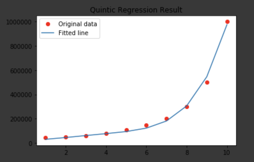
Quintic

with tf.Session() as sess:
    sess.run(init)
    for epoch in range(no_of_epochs):
      for (x,y) in zip(abscissa, ordinate):
        sess.run(optimizer5, feed_dict={X:x, Y:y})
      if (epoch+1)%1000==0:
        cost = sess.run(mse5,feed_dict={X:abscissa,Y:ordinate})
        print("Epoch",(epoch+1), ": Training Cost:", cost," a,b,c,d,e,f:",sess.run(a),sess.run(b),sess.run(c),sess.run(d),sess.run(e),sess.run(f))

        training_cost = sess.run(mse5,feed_dict={X:abscissa,Y:ordinate})
        coefficient1 = sess.run(a)
        coefficient2 = sess.run(b)
        coefficient3 = sess.run(c)
        coefficient4 = sess.run(d)
        coefficient5 = sess.run(e)
        constant = sess.run(f)

Epoch 1000 : Training Cost: 1409200100.0  a,b,c,d,e,f: 7.949472 7.46219 55.626034 184.29028 484.00223 1024.0083
Epoch 2000 : Training Cost: 1306882400.0  a,b,c,d,e,f: 8.732181 -4.0085897 73.25298 315.90103 904.08887 2004.9749
Epoch 3000 : Training Cost: 1212606000.0  a,b,c,d,e,f: 9.732249 -16.90125 86.28379 437.06552 1305.055 2966.2188
Epoch 4000 : Training Cost: 1123640400.0  a,b,c,d,e,f: 10.74851 -29.82692 98.59997 555.331 1698.4631 3917.9155
Epoch 5000 : Training Cost: 1039694300.0  a,b,c,d,e,f: 11.75426 -42.598194 110.698326 671.64355 2085.5513 4860.8535
Epoch 6000 : Training Cost: 960663550.0  a,b,c,d,e,f: 12.745439 -55.18337 122.644936 786.00214 2466.1638 5794.3735
Epoch 7000 : Training Cost: 886438340.0  a,b,c,d,e,f: 13.721028 -67.57168 134.43822 898.3691 2839.9958 6717.659
Epoch 8000 : Training Cost: 816913100.0  a,b,c,d,e,f: 14.679965 -79.75113 146.07385 1008.66895 3206.6692 7629.812
Epoch 9000 : Training Cost: 751971500.0  a,b,c,d,e,f: 15.62181 -91.71608 157.55713 1116.7715 3565.8323 8529.976
Epoch 10000 : Training Cost: 691508740.0  a,b,c,d,e,f: 16.545347 -103.4531 168.88321 1222.6348 3916.9785 9416.236
Epoch 11000 : Training Cost: 635382000.0  a,b,c,d,e,f: 17.450052 -114.954254 180.03932 1326.1565 4259.842 10287.99
Epoch 12000 : Training Cost: 583477250.0  a,b,c,d,e,f: 18.334944 -126.20821 191.02948 1427.2095 4593.8 11143.449
Epoch 13000 : Training Cost: 535640400.0  a,b,c,d,e,f: 19.198917 -137.20206 201.84718 1525.6926 4918.5327 11981.633
Epoch 14000 : Training Cost: 491722240.0  a,b,c,d,e,f: 20.041153 -147.92719 212.49709 1621.5496 5233.627 12800.468
Epoch 15000 : Training Cost: 451559520.0  a,b,c,d,e,f: 20.860966 -158.37456 222.97133 1714.7141 5538.676 13598.337
Epoch 16000 : Training Cost: 414988960.0  a,b,c,d,e,f: 21.657421 -168.53406 233.27422 1805.0874 5833.1978 14373.658
Epoch 17000 : Training Cost: 381837920.0  a,b,c,d,e,f: 22.429693 -178.39536 243.39914 1892.5883 6116.847 15124.394
Epoch 18000 : Training Cost: 351931300.0  a,b,c,d,e,f: 23.176882 -187.94789 253.3445 1977.137 6389.117 15848.417
Epoch 19000 : Training Cost: 325074400.0  a,b,c,d,e,f: 23.898485 -197.18741 263.12512 2058.6716 6649.8037 16543.95
Epoch 20000 : Training Cost: 301073570.0  a,b,c,d,e,f: 24.593851 -206.10497 272.72385 2137.1797 6898.544 17209.367
Epoch 21000 : Training Cost: 279727000.0  a,b,c,d,e,f: 25.262104 -214.69217 282.14642 2212.6372 7135.217 17842.854
Epoch 22000 : Training Cost: 260845550.0  a,b,c,d,e,f: 25.903376 -222.94969 291.4003 2284.9844 7359.4644 18442.408
Epoch 23000 : Training Cost: 244218030.0  a,b,c,d,e,f: 26.517094 -230.8697 300.45532 2354.3003 7571.261 19007.49
Epoch 24000 : Training Cost: 229660080.0  a,b,c,d,e,f: 27.102589 -238.44817 309.35342 2420.4185 7770.5728 19536.19
Epoch 25000 : Training Cost: 216972400.0  a,b,c,d,e,f: 27.660324 -245.69016 318.10062 2483.3608 7957.354 20027.707
216972400.0 27.660324 -245.69016 318.10062 2483.3608 7957.354 20027.707

predictions = []
for x in abscissa:
  predictions.append((coefficient1*pow(x,5) + coefficient2*pow(x,4) + coefficient3*pow(x,3) + coefficient4*pow(x,2) + coefficient5*x + constant))
plt.plot(abscissa , ordinate, 'ro', label ='Original data')
plt.plot(abscissa, predictions, label ='Fitted line')
plt.title('Quintic Regression Result')
plt.legend()
plt.show()

Results and Conclusion

You just learnt Polynomial Regression using TensorFlow!

Notes

Overfitting

Overfitting refers to a model that models the training data too well. Overfitting happens when a model learns the detail and noise in the training data to the extent that it negatively impacts the performance of the model on new data. This means that the noise or random fluctuations in the training data is picked up and learned as concepts by the model. The problem is that these concepts do not apply to new data and negatively impact the models ability to generalise.

Source: Machine Learning Mastery

Basically if you train your machine learning model on a small dataset for a really large number of epochs, the model will learn all the deformities/noise in the data and will actually think that it is a normal part. Therefore when it will see some new data, it will discard that new data as noise and will impact the accuracy of the model in a negative manner

Navan